Joining data from multiple sourcesBecky Tang05.24.20211

`mutate`

(from May 20 lecture)

`mutate` to add new variables

hotels %>% 
  mutate(people = adults + babies + children)

"Save" when you `mutate`

Most often when you define a new variable with mutate you'll also want to save the resulting data frame, often by writing over the original data frame.

hotels <- hotels %>% 
  mutate(people = adults + babies + children)

Check before you move on

hotels %>% 
  select(adults, children,babies, people)

## # A tibble: 119,390 x 4
##    adults children babies people
##     <dbl>    <dbl>  <dbl>  <dbl>
##  1      2        0      0      2
##  2      2        0      0      2
##  3      1        0      0      1
##  4      1        0      0      1
##  5      2        0      0      2
##  6      2        0      0      2
##  7      2        0      0      2
##  8      2        0      0      2
##  9      2        0      0      2
## 10      2        0      0      2
## # … with 119,380 more rows

Working with multiple data frames

Fisheries of the world

Fisheries and Aquaculture Department of the Food and Agriculture Organization of the United Nations collects data on fisheries production of countries.

...

Source: https://en.wikipedia.org/wiki/Fishing_industry_by_country

Load data

fisheries <- read_csv("data/fisheries.csv")

First look at the data

glimpse(fisheries)

## Rows: 216
## Columns: 4
## $ country     <chr> "Afghanistan", "Albania", "Algeria", "American Samoa", "An…
## $ capture     <dbl> 1000, 7886, 95000, 3047, 0, 486490, 3000, 755226, 3758, 14…
## $ aquaculture <dbl> 1200, 950, 1361, 20, 0, 655, 10, 3673, 16381, 0, 96847, 34…
## $ total       <dbl> 2200, 8836, 96361, 3067, 0, 487145, 3010, 758899, 20139, 1…

Quick summaries of the data

skim(fisheries) #skimr package

## ── Data Summary ────────────────────────
##                            Values   
## Name                       fisheries
## Number of rows             216      
## Number of columns          4        
## _______________________             
## Column type frequency:              
##   character                1        
##   numeric                  3        
## ________________________            
## Group variables            None     
## 
## ── Variable type: character ────────────────────────────────────────────────────────────────────────────────────────────────────────────────
##   skim_variable n_missing complete_rate   min   max empty n_unique whitespace
## 1 country               0             1     4    32     0      215          0
## 
## ── Variable type: numeric ──────────────────────────────────────────────────────────────────────────────────────────────────────────────────
##   skim_variable n_missing complete_rate    mean       sd    p0    p25    p50     p75     p100 hist 
## 1 capture               0             1 421916. 1478638.     0 3280.  33797  221884. 17800000 ▇▁▁▁▁
## 2 aquaculture           0             1 508368. 4496073.     0   25.2  1574.  25998  63700000 ▇▁▁▁▁
## 3 total                 0             1 930284. 5846301.     0 7270.  44648. 271901. 81500000 ▇▁▁▁▁

Some summary stats

fisheries %>%
  summarise(
    mean_cap = mean(capture),
    mean_aqc = mean(aquaculture),
    mean_tot = mean(total)
  )

## # A tibble: 1 x 3
##   mean_cap mean_aqc mean_tot
##      <dbl>    <dbl>    <dbl>
## 1  421916.  508368.  930284.

Some summary stats

fisheries %>%
  summarise(
    mean_cap = mean(capture),
    mean_aqc = mean(aquaculture),
    mean_tot = mean(total)
  )

## # A tibble: 1 x 3
##   mean_cap mean_aqc mean_tot
##      <dbl>    <dbl>    <dbl>
## 1  421916.  508368.  930284.

well, that was boring...

A new approach!

fisheries %>%
  summarise(across(capture:total, mean))

## # A tibble: 1 x 3
##   capture aquaculture   total
##     <dbl>       <dbl>   <dbl>
## 1 421916.     508368. 930284.

The (not-so-great) visualization below shows the distribution of fishery harvest of countries for 2016, by capture and aquaculture. What are some ways you would improve this visualization? Note that countries whose total harvest was less than 100,000 tons are not included in the visualization.

Goal: calculate summary statistics at the continent level and visualize them

Data prep

continents <- read_csv("data/continents.csv")

Data prep

continents <- read_csv("data/continents.csv")

Filter out countries whose total harvest was less than 100,000 tons since they are not included in the visualization:

fisheries <- fisheries %>%
  filter(total >= 100000)
fisheries

## # A tibble: 82 x 4
##    country    capture aquaculture   total
##    <chr>        <dbl>       <dbl>   <dbl>
##  1 Angola      486490         655  487145
##  2 Argentina   755226        3673  758899
##  3 Australia   174629       96847  271476
##  4 Bangladesh 1674770     2203554 3878324
##  5 Brazil      705000      581230 1286230
##  6 Cambodia    629950      172500  802450
##  7 Cameroon    233190        2315  235505
##  8 Canada      874727      200765 1075492
##  9 Chad        110000          94  110094
## 10 Chile      1829238     1050117 2879355
## # … with 72 more rows

Data joins

fisheries %>% select(country)

## # A tibble: 82 x 1
##    country   
##    <chr>     
##  1 Angola    
##  2 Argentina 
##  3 Australia 
##  4 Bangladesh
##  5 Brazil    
##  6 Cambodia  
##  7 Cameroon  
##  8 Canada    
##  9 Chad      
## 10 Chile     
## # … with 72 more rows

continents

## # A tibble: 245 x 2
##    country           continent
##    <chr>             <chr>    
##  1 Afghanistan       Asia     
##  2 Åland Islands     Europe   
##  3 Albania           Europe   
##  4 Algeria           Africa   
##  5 American Samoa    Oceania  
##  6 Andorra           Europe   
##  7 Angola            Africa   
##  8 Anguilla          Americas 
##  9 Antigua & Barbuda Americas 
## 10 Argentina         Americas 
## # … with 235 more rows

Joining data frames

something_join(x, y)

Mutating joins:

inner_join(): all rows from x where there are matching values in y, return all combination of multiple matches in the case of multiple matches
left_join(): all rows from x
right_join(): all rows from y
full_join(): all rows from both x and y

Filtering joins:

semi_join(): all rows from x where there are matching values in y, keeping just columns from x.
anti_join(): return all rows from x where there are not matching values in y, never duplicate rows of x
...

Setup

For the next few slides...

## # A tibble: 3 x 1
##   value
##   <dbl>
## 1     1
## 2     2
## 3     3

## # A tibble: 3 x 1
##   value
##   <dbl>
## 1     1
## 2     2
## 3     4

`inner_join()`

Adds columns to x from y, matching all rows in x AND y

inner_join(x, y)

## # A tibble: 2 x 1
##   value
##   <dbl>
## 1     1
## 2     2

`left_join()`

Adds columns to x from y, matching all rows in x

left_join(x, y)

## # A tibble: 3 x 1
##   value
##   <dbl>
## 1     1
## 2     2
## 3     3

`right_join()`

Adds columns to x from y, matching all rows in y

right_join(x, y)

## # A tibble: 3 x 1
##   value
##   <dbl>
## 1     1
## 2     2
## 3     4

`full_join()`

Adds columns to x from y, matching all rows in x OR y

full_join(x, y)

## # A tibble: 4 x 1
##   value
##   <dbl>
## 1     1
## 2     2
## 3     3
## 4     4

`semi_join()`

Returns all rows from x with a match in y (does not add columns from y)

semi_join(x, y)

## # A tibble: 2 x 1
##   value
##   <dbl>
## 1     1
## 2     2

`anti_join()`

Returns all rows from x without a match in y (does not add columns from y)

anti_join(x, y)

## # A tibble: 1 x 1
##   value
##   <dbl>
## 1     3

We want to keep all rows and columns from fisheries and add a column for corresponding continents. Which join function should we use?

fisheries %>% select(country)

## # A tibble: 82 x 1
##    country   
##    <chr>     
##  1 Angola    
##  2 Argentina 
##  3 Australia 
##  4 Bangladesh
##  5 Brazil    
##  6 Cambodia  
##  7 Cameroon  
##  8 Canada    
##  9 Chad      
## 10 Chile     
## # … with 72 more rows

continents

## # A tibble: 245 x 2
##    country           continent
##    <chr>             <chr>    
##  1 Afghanistan       Asia     
##  2 Åland Islands     Europe   
##  3 Albania           Europe   
##  4 Algeria           Africa   
##  5 American Samoa    Oceania  
##  6 Andorra           Europe   
##  7 Angola            Africa   
##  8 Anguilla          Americas 
##  9 Antigua & Barbuda Americas 
## 10 Argentina         Americas 
## # … with 235 more rows

Join fisheries and continents

fisheries <- left_join(fisheries, continents)

Join fisheries and continents

fisheries <- left_join(fisheries, continents)

How does left_join() know to join the two data frames by country?

Hint:

Variables in the original fisheries dataset:

## [1] "country"     "capture"     "aquaculture" "total"

Variables in the continents dataset:

## [1] "country"   "continent"

Check the data

fisheries %>%
  slice(11:20)

## # A tibble: 10 x 5
##    country                           capture aquaculture    total continent
##    <chr>                               <dbl>       <dbl>    <dbl> <chr>    
##  1 China                            17800000    63700000 81500000 Asia     
##  2 Colombia                            86344       96970   183314 Americas 
##  3 Democratic Republic of the Congo   237372        3161   240533 <NA>     
##  4 Denmark                            670344       36337   706681 Europe   
##  5 Ecuador                            715495      451090  1166585 Americas 
##  6 Egypt                              335614     1370660  1706274 Africa   
##  7 Faroe Islands                      568435       83300   651735 Europe   
##  8 Finland                            192065       14412   206477 Europe   
##  9 France                             561173      166640   727813 Europe   
## 10 Germany                            271185       41721   312906 Europe

Check the data

fisheries %>%
  filter(is.na(continent))

## # A tibble: 3 x 5
##   country                          capture aquaculture   total continent
##   <chr>                              <dbl>       <dbl>   <dbl> <chr>    
## 1 Democratic Republic of the Congo  237372        3161  240533 <NA>     
## 2 Hong Kong                         142775        4258  147033 <NA>     
## 3 Myanmar                          2072390     1017644 3090034 <NA>

Implement fixes

fisheries <- fisheries %>%
  mutate(continent = case_when(
    country == "Democratic Republic of the Congo" ~ "Africa",
    country == "Hong Kong"                        ~ "Asia",
    country == "Myanmar"                          ~ "Asia",
    TRUE                                          ~ continent
    )
  )

...and check again

fisheries %>%
  filter(is.na(continent))

## # A tibble: 0 x 5
## # … with 5 variables: country <chr>, capture <dbl>, aquaculture <dbl>, total <dbl>,
## #   continent <chr>

What does the following code do?

fisheries %>%
  mutate(aquaculture_perc = aquaculture / total)

Demo

Visualize continent summary stats

ggplot(fisheries_summary, aes(x = continent, y = mean_ap)) +
  geom_col()

Improve visualization

ggplot(fisheries_summary, 
       aes(x = fct_reorder(continent, mean_ap), y = mean_ap)) +
  geom_col()

Improve visualization further

ggplot(fisheries_summary, 
       aes(y = fct_reorder(continent, mean_ap), x = mean_ap)) +
  geom_col() +
  labs(
    x = "",
    y = "",
    title = "Average share of aquaculture by continent",
    subtitle = "out of total fisheries harvest, 2016",
    caption = "Source: bit.ly/2VrawTt"
  ) +
  theme_minimal()

↑, ←, Pg Up, k	Go to previous slide
↓, →, Pg Dn, Space, j	Go to next slide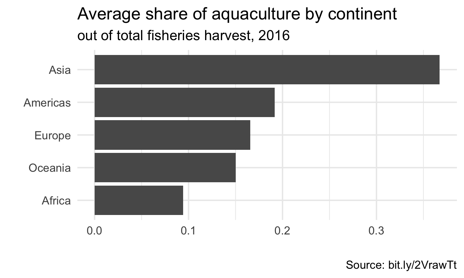
Home	Go to first slide
End	Go to last slide
Number + Return	Go to specific slide
b / m / f	Toggle blackout / mirrored / fullscreen mode
c	Clone slideshow
p	Toggle presenter mode
t	Restart the presentation timer
?, h	Toggle this help

Joining data from multiple sources

Becky Tang

05.24.2021

mutate

mutate to add new variables

"Save" when you mutate

Check before you move on

Working with multiple data frames

Fisheries of the world

Load data

First look at the data

Quick summaries of the data

Some summary stats

Some summary stats

A new approach!

Goal: calculate summary statistics at the continent level and visualize them

Data prep

Data prep

Data joins

Joining data frames

Setup

inner_join()

left_join()

right_join()

full_join()

semi_join()

anti_join()

Join fisheries and continents

Join fisheries and continents

Check the data

Check the data

Implement fixes

Demo

Demo

Visualize continent summary stats

Improve visualization

Improve visualization further

mutate

Help

`mutate`

`mutate` to add new variables

"Save" when you `mutate`

`inner_join()`

`left_join()`

`right_join()`

`full_join()`

`semi_join()`

`anti_join()`

`mutate`